
ABOUT THE COURSE :
Deep Learning has received a lot of attention over the past few years and has been employed successfully by companies like Google, Microsoft, IBM, Facebook, Twitter etc. to solve a wide range of problems in Computer Vision and Natural Language Processing. In this course we will learn about the building blocks used in these Deep Learning based solutions. Specifically, we will learn about feedforward neural networks, convolutional neural networks, recurrent neural networks and attention mechanisms. We will also look at various optimization algorithms such as Gradient Descent, Nesterov Accelerated Gradient Descent, Adam, AdaGrad and RMSProp which are used for training such deep neural networks. At the end of this course students would have knowledge of deep architectures used for solving various Vision and NLP tasks
Deep Learning has received a lot of attention over the past few years and has been employed successfully by companies like Google, Microsoft, IBM, Facebook, Twitter etc. to solve a wide range of problems in Computer Vision and Natural Language Processing. In this course we will learn about the building blocks used in these Deep Learning based solutions. Specifically, we will learn about feedforward neural networks, convolutional neural networks, recurrent neural networks and attention mechanisms. We will also look at various optimization algorithms such as Gradient Descent, Nesterov Accelerated Gradient Descent, Adam, AdaGrad and RMSProp which are used for training such deep neural networks. At the end of this course students would have knowledge of deep architectures used for solving various Vision and NLP tasks
INTENDED AUDIENCE: Any Interested Learners
PREREQUISITES: Working knowledge of Linear Algebra, Probability Theory. It would be beneficial if the participants have done a course on Machine Learning.
Nptel Deep Learning – IIT Ropar Week 3 Assignment Answer
Course layout
Week 1 : (Partial) History of Deep Learning, Deep Learning Success Stories, McCulloch Pitts Neuron, Thresholding Logic, Perceptrons, Perceptron Learning Algorithm
Week 2 : Multilayer Perceptrons (MLPs), Representation Power of MLPs, Sigmoid Neurons, Gradient Descent, Feedforward Neural Networks, Representation Power of Feedforward Neural Networks
Week 3 : FeedForward Neural Networks, Backpropagation
Week 4 : Gradient Descent (GD), Momentum Based GD, Nesterov Accelerated GD, Stochastic GD, AdaGrad, RMSProp, Adam, Eigenvalues and eigenvectors, Eigenvalue Decomposition, Basis
Week 5 : Principal Component Analysis and its interpretations, Singular Value Decomposition
Week 6 : Autoencoders and relation to PCA, Regularization in autoencoders, Denoising autoencoders, Sparse autoencoders, Contractive autoencoders
Week 7 : Regularization: Bias Variance Tradeoff, L2 regularization, Early stopping, Dataset augmentation, Parameter sharing and tying, Injecting noise at input, Ensemble methods, Dropout
Week 8 : Greedy Layerwise Pre-training, Better activation functions, Better weight initialization methods, Batch Normalization
Week 9 : Learning Vectorial Representations Of Words
Week 10: Convolutional Neural Networks, LeNet, AlexNet, ZF-Net, VGGNet, GoogLeNet, ResNet, Visualizing Convolutional Neural Networks, Guided Backpropagation, Deep Dream, Deep Art, Fooling Convolutional Neural Networks
Week 11: Recurrent Neural Networks, Backpropagation through time (BPTT), Vanishing and Exploding Gradients, Truncated BPTT, GRU, LSTMs
Week 12: Encoder Decoder Models, Attention Mechanism, Attention over images
Nptel Deep Learning – IIT Ropar Week 3 Assignment Answer
Week 3 : Assignment 3
Due date: 2025-02-12, 23:59 IST.
Assignment not submitted
Use the following data to answer the questions 1 to 2
A neural network contains an input layer h0=xh0=x, three hidden layers (h1,h2,h3),(h1,h2,h3), and an output layer O. All the hidden layers use the Sigmoid activation function, and the output layer uses the Softmax activation function.
Suppose the input x∈R200x∈R200, and all the hidden layers contain 10 neurons each. The output layer contains 4 neurons.
1 point
1 point
Use the following data to answer the questions 3 to 4
The diagram below shows a neural network. The network contains two hidden layers and one output layer. The input to the network is a column vector x∈R3x∈R3. The first hidden layer contains 9 neurons, the second hidden layer contains 5 neurons and the output layer contains 2 neurons. Each neuron in the lthlth layer is connected to all the neurons in the (l+1)th(l+1)th layer. Each neuron has a bias connected to it (not explicitly shown in the figure)
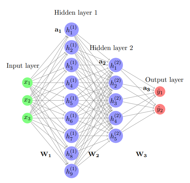
In the diagram, W1W1 is a matrix and x,a1,h1,x,a1,h1, and OO are all column vectors. The notation Wi[j,:]Wi[j,:] denotes the jthjth row of the matrix Wi,Wi[:,j]Wi,Wi[:,j] denotes the jthjth column of the matrix WiWi and WkijWkij denotes an element at ithith row and jthjth column of the matrix WkWk.
The diagram below shows a neural network. The network contains two hidden layers and one output layer. The input to the network is a column vector x∈R3x∈R3. The first hidden layer contains 9 neurons, the second hidden layer contains 5 neurons and the output layer contains 2 neurons. Each neuron in the lthlth layer is connected to all the neurons in the (l+1)th(l+1)th layer. Each neuron has a bias connected to it (not explicitly shown in the figure)
In the diagram, W1W1 is a matrix and x,a1,h1,x,a1,h1, and OO are all column vectors. The notation Wi[j,:]Wi[j,:] denotes the jthjth row of the matrix Wi,Wi[:,j]Wi,Wi[:,j] denotes the jthjth column of the matrix WiWi and WkijWkij denotes an element at ithith row and jthjth column of the matrix WkWk.
1 point
Use the following data to answer the questions 9 and 10
The following diagram represents a neural network containing two hidden layers and one output layer. The input to the network is a column vector x∈R3.x∈R3. The activation function used in hidden layers is sigmoid. The output layer doesn’t contain any activation function and the loss used is squared error loss (predy−truey)2.(predy−truey)2.
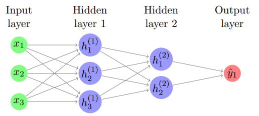
The following network doesn’t contain any biases and the weights of the network are given below:
W1=⎡⎣⎢1211−1231−2⎤⎦⎥W2=[131121]W3=[12]W1=[1132−1112−2]W2=[112311]W3=[12]
The input to the network is: x=⎡⎣⎢121⎤⎦⎥x=[121]
The target value y is: y=5y=5
The following diagram represents a neural network containing two hidden layers and one output layer. The input to the network is a column vector x∈R3.x∈R3. The activation function used in hidden layers is sigmoid. The output layer doesn’t contain any activation function and the loss used is squared error loss (predy−truey)2.(predy−truey)2.
The following network doesn’t contain any biases and the weights of the network are given below:
W1=⎡⎣⎢1211−1231−2⎤⎦⎥W2=[131121]W3=[12]W1=[1132−1112−2]W2=[112311]W3=[12]
The input to the network is: x=⎡⎣⎢121⎤⎦⎥x=[121]
The target value y is: y=5y=5
1 point